Reconstructing an RC F maneuver from video
I wanted to see how much I could reconstruct from a short cabin video of my friend’s 2016 Lexus RC F pulling out at E Brooklyn Village Avenue and S Brevard Street in Charlotte. I built a replay that combines the original footage, tracked image features, official map records and a model of plausible vehicle motion.
The result is a best estimate with editable assumptions. The original detections and failed checks remain available alongside it.
The replay keeps recorded image features separate from estimated motion. Amber marks the modeled 7.4–10.6 second interval.
Start with the frames
The uploaded MOV contains 449 decoded frames, with presentation timestamps spaced at 1/30 second. Its browser duration is 14.97 seconds. The portrait presentation is 2160 × 3840; I used a 540 × 960 derivative for the initial analysis. The embedded video is a smaller 720p copy with the same frame timing and stripped container metadata.
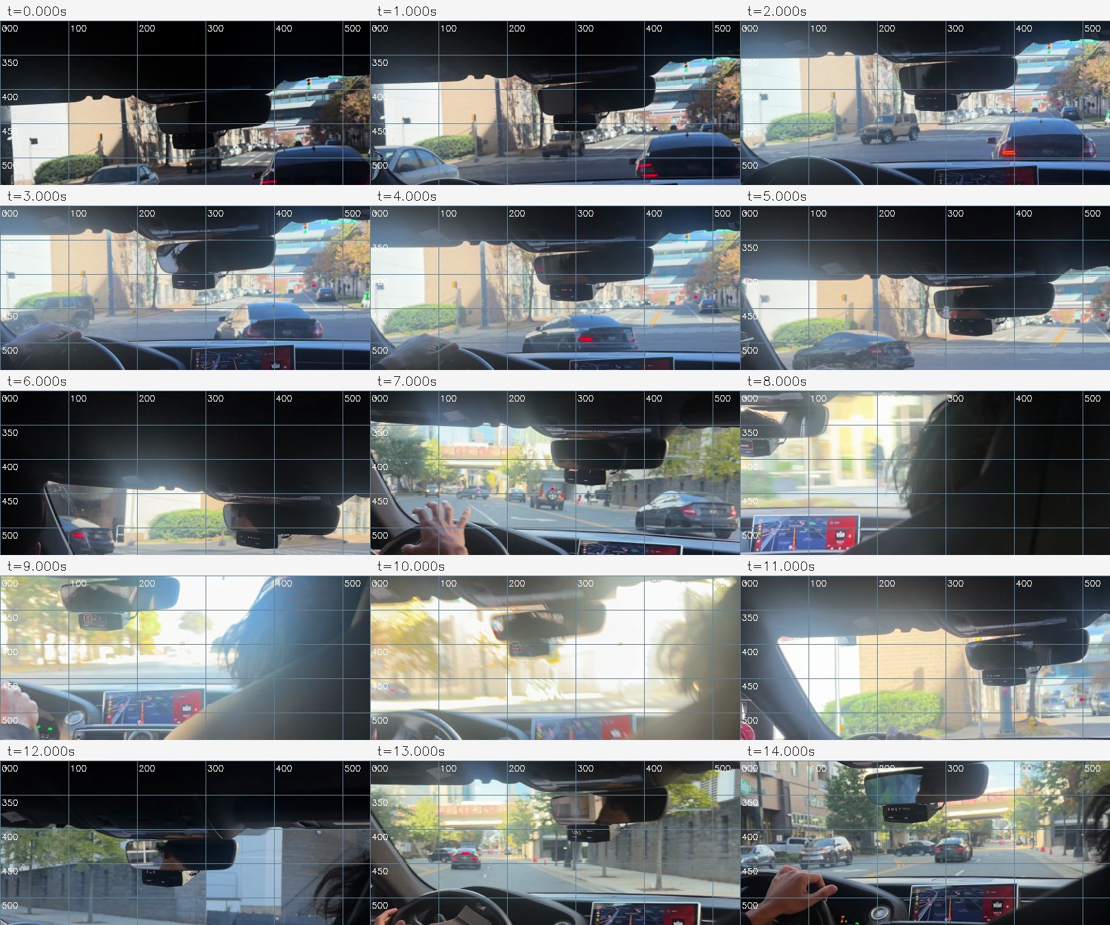
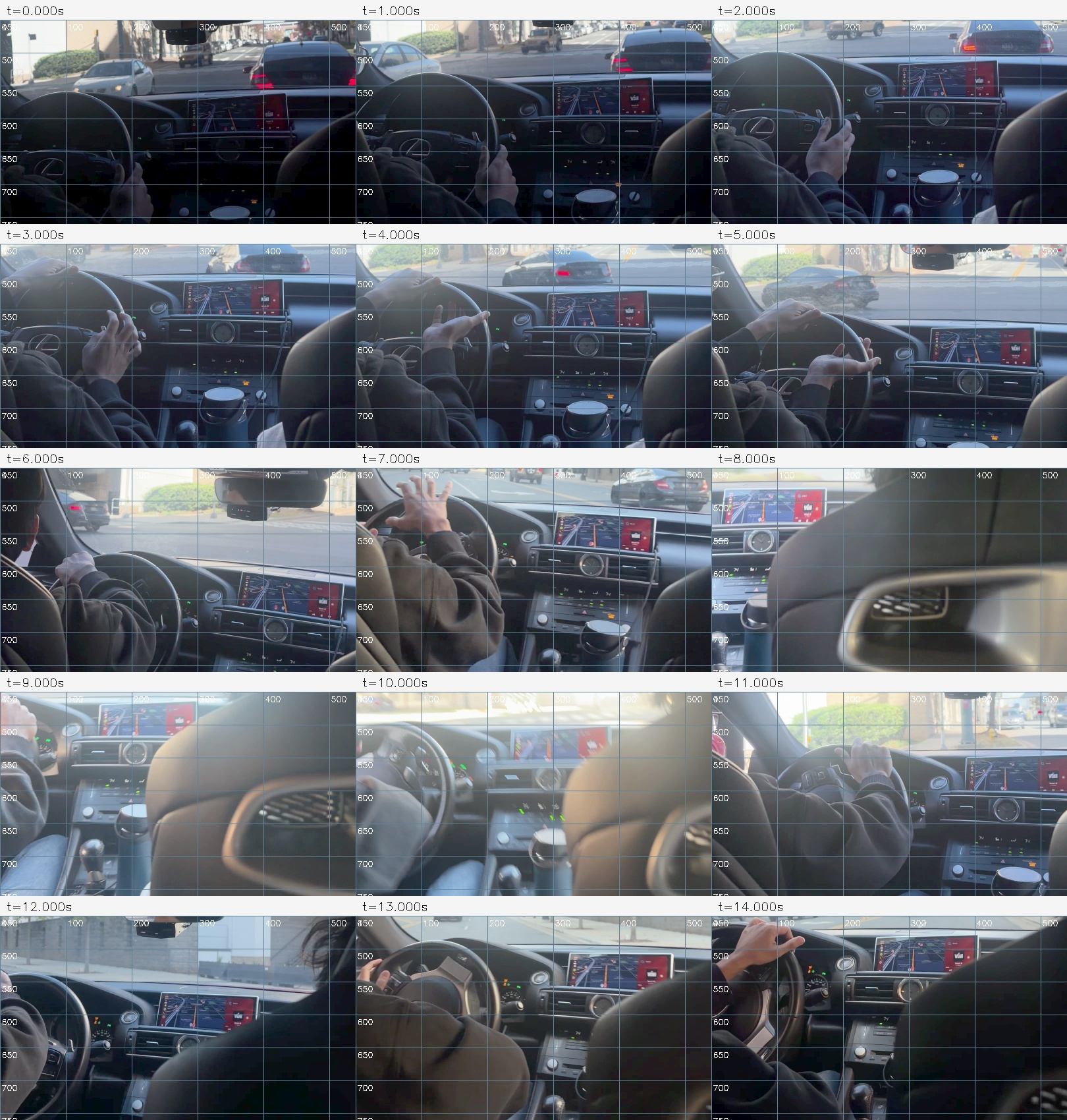
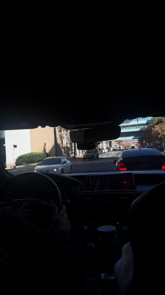
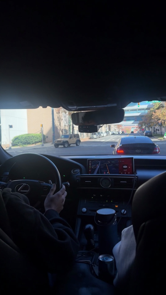
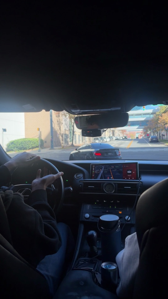
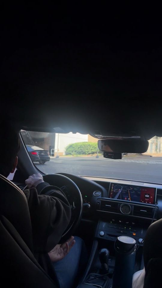
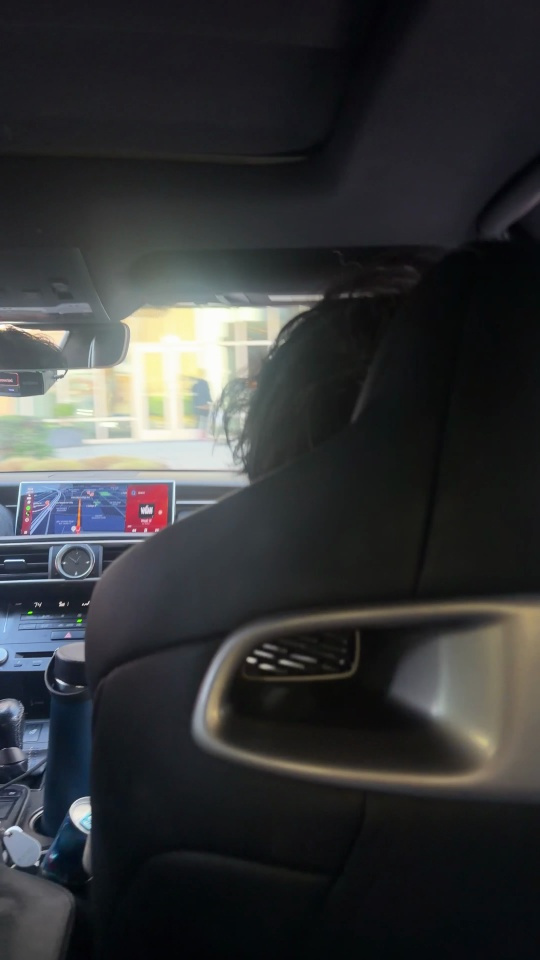
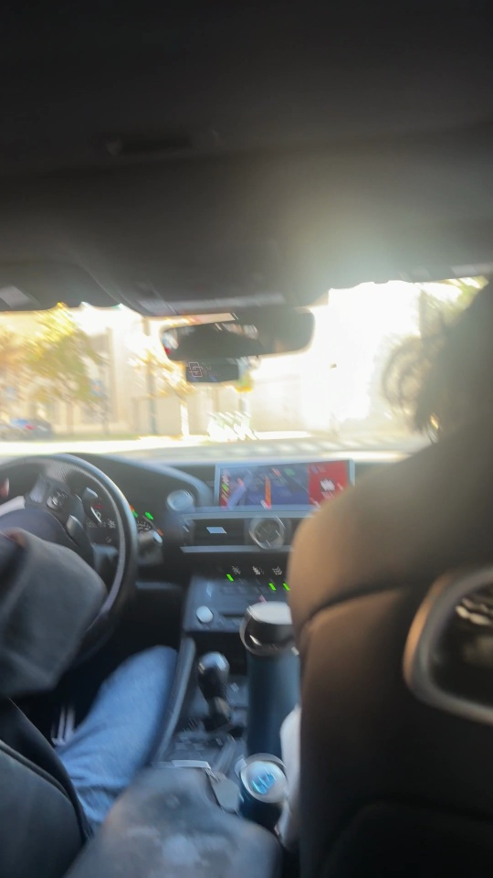
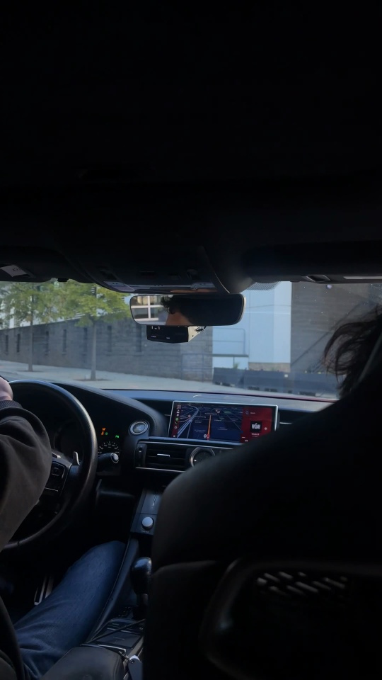
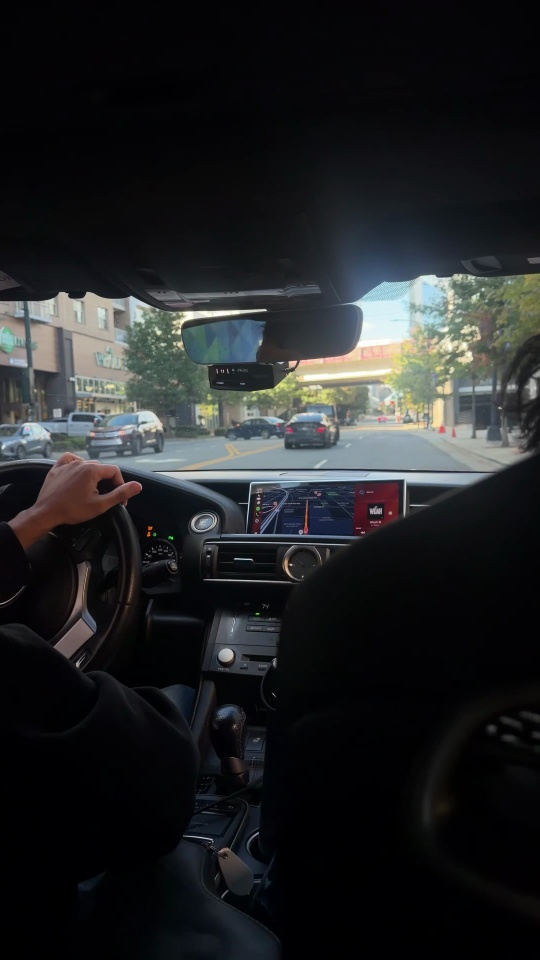
I first checked the footage as a contact sheet, then inspected larger wheel and windshield crops. The view changes substantially during the clip. Hands cover the steering wheel, the phone moves, and the passenger and glare obscure much of 7.4–10.6 seconds.
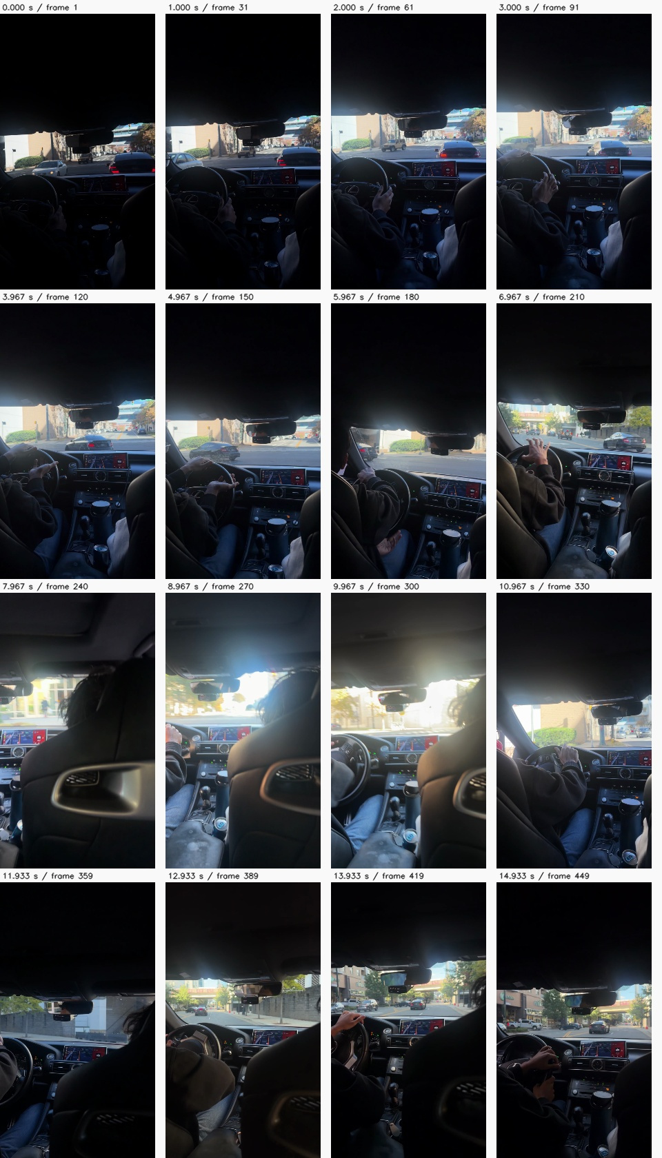
Wheel, windshield and larger sampled frames
Give the map a scale
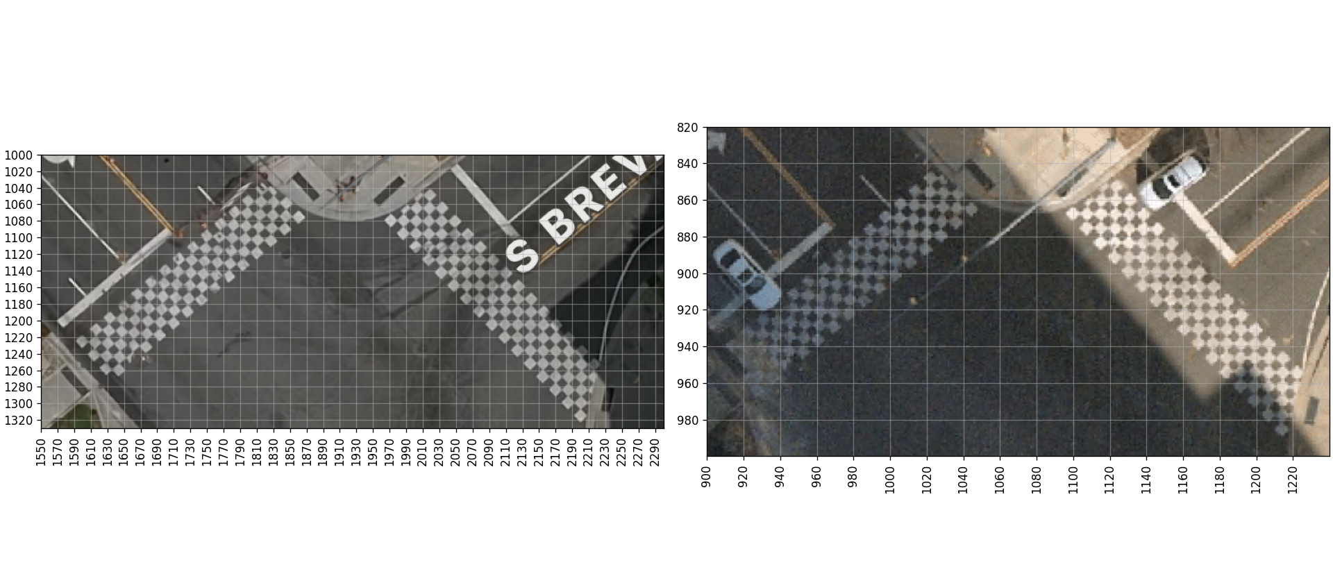
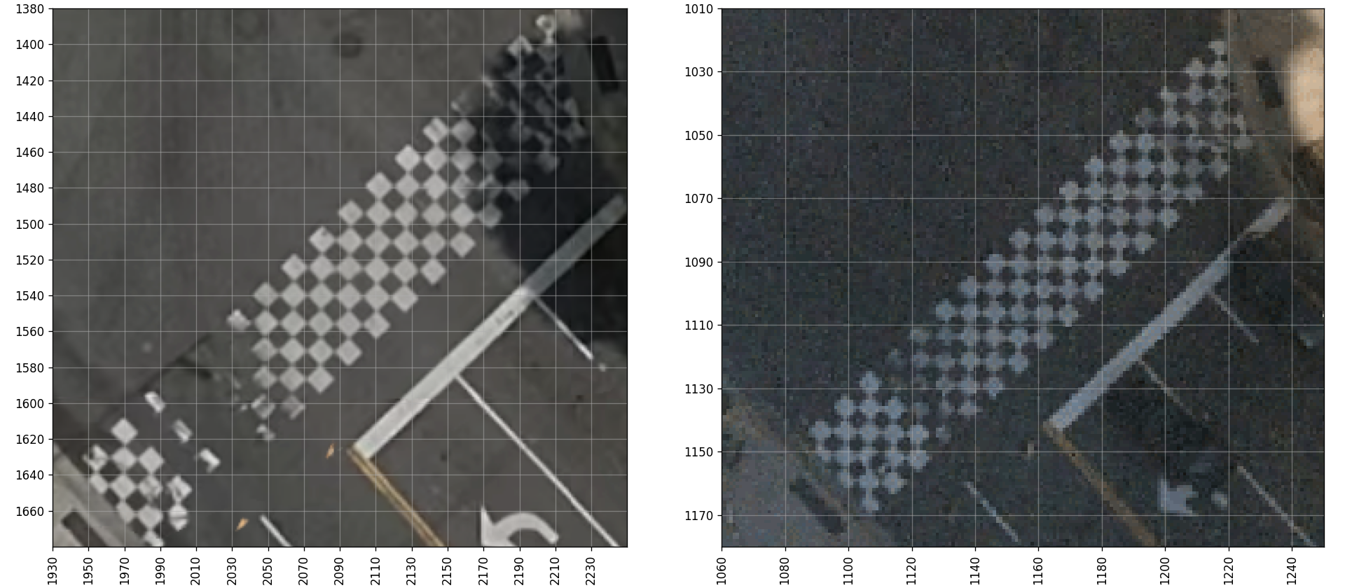
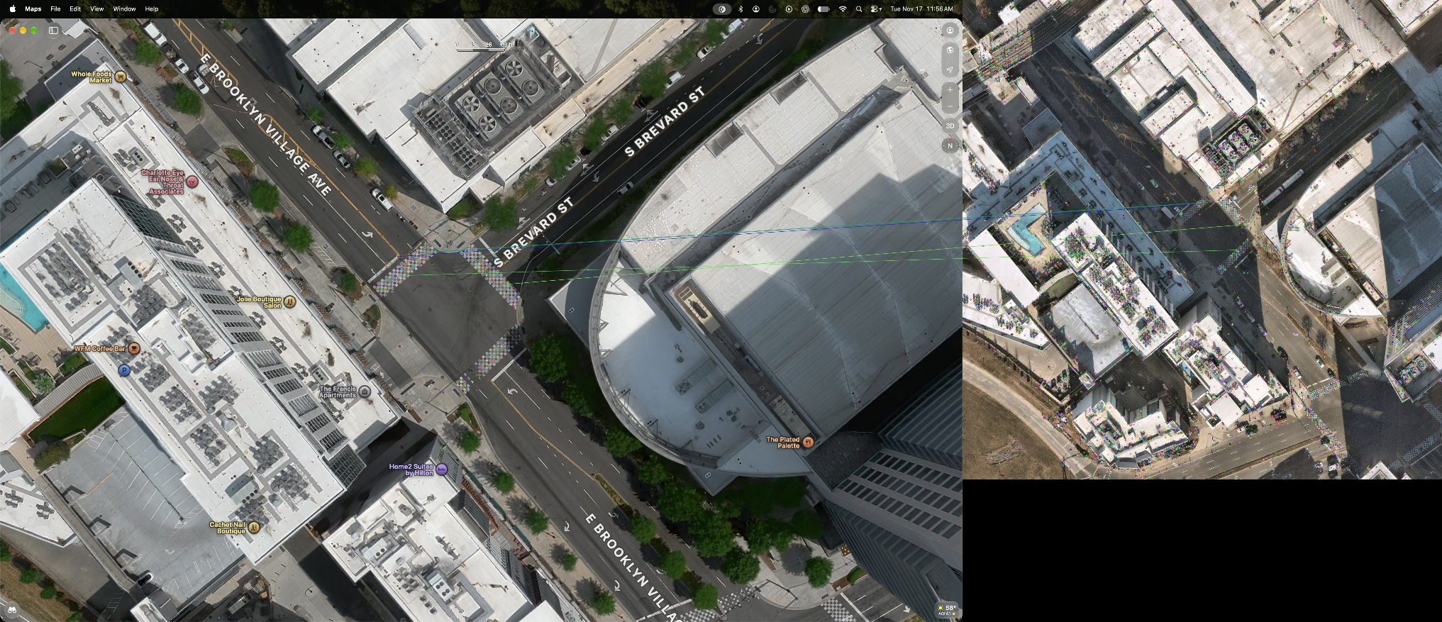
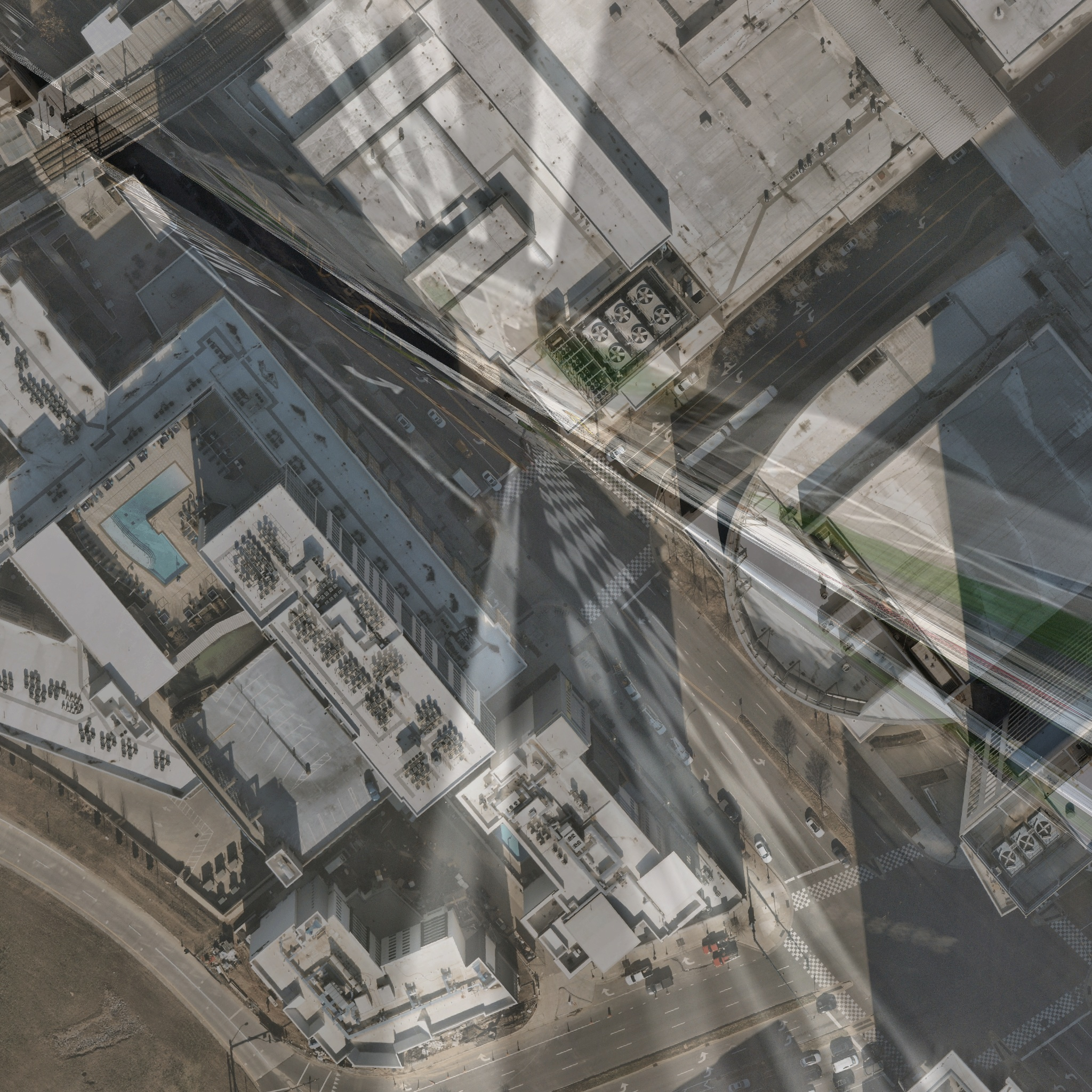
I used my Apple Maps screenshot as the visual reference and retrieved the 2024 aerial from the City of Charlotte’s public ArcGIS service. A street-intersection geocoder placed the junction at approximately 35.220756, −80.845538. The export records its extent and Web Mercator coordinate system. Transforming that grid to local UTM metres gave about 0.112 m per aerial pixel near the intersection.
Automatic image matching was unreliable here. The first SIFT fit had only six inliers, including a duplicate and an implausible match. I rejected it and picked ground-paint controls manually.
Six controls gave a 0.57 m fit RMS. Two separate check points differed by 1.26 m and 1.29 m. Those errors describe the overhead alignment. Manual selection, changed markings and source geolocation add uncertainty to any vehicle placement.
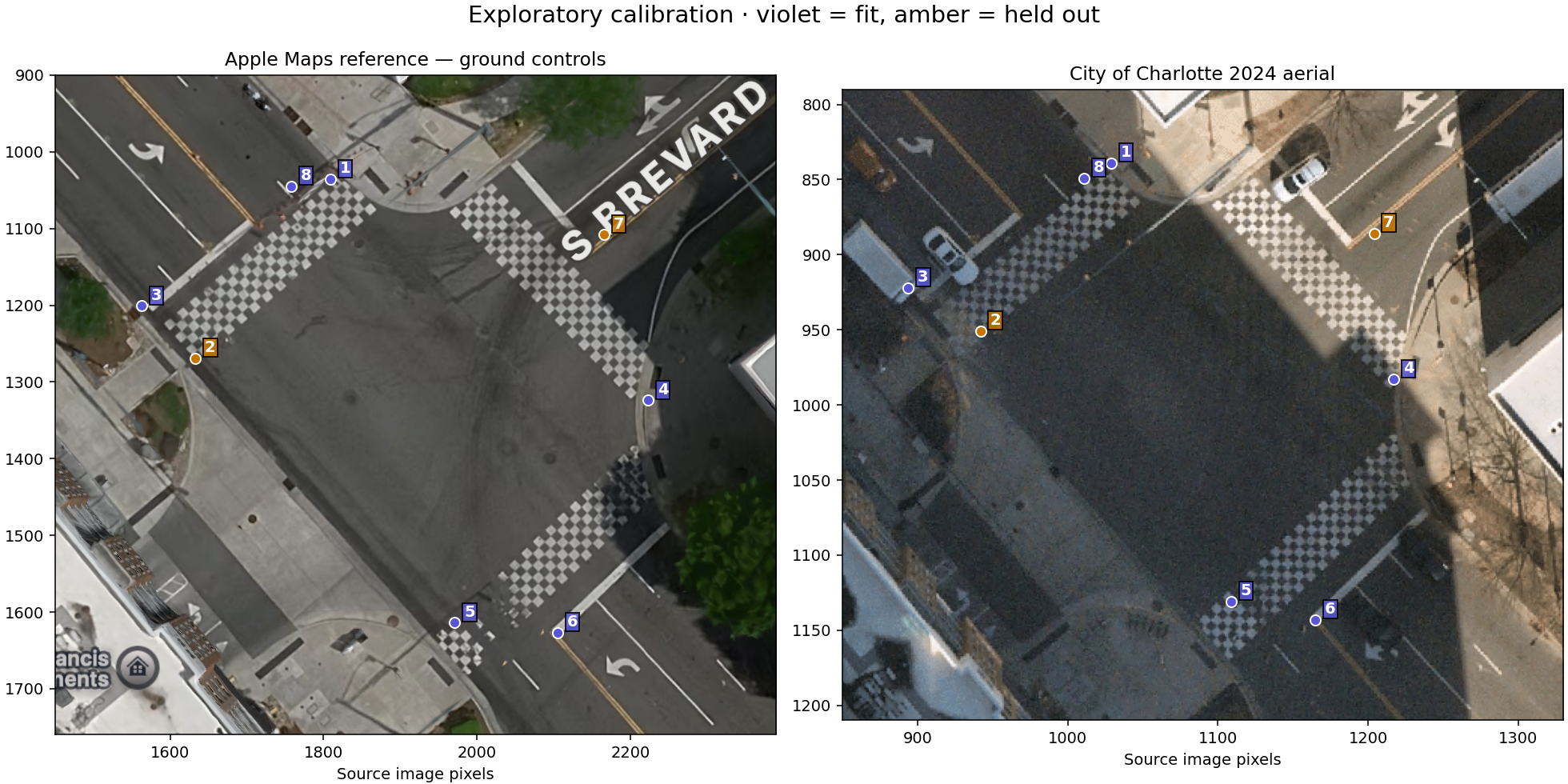
Map inputs, coordinate grids and rejected alignment
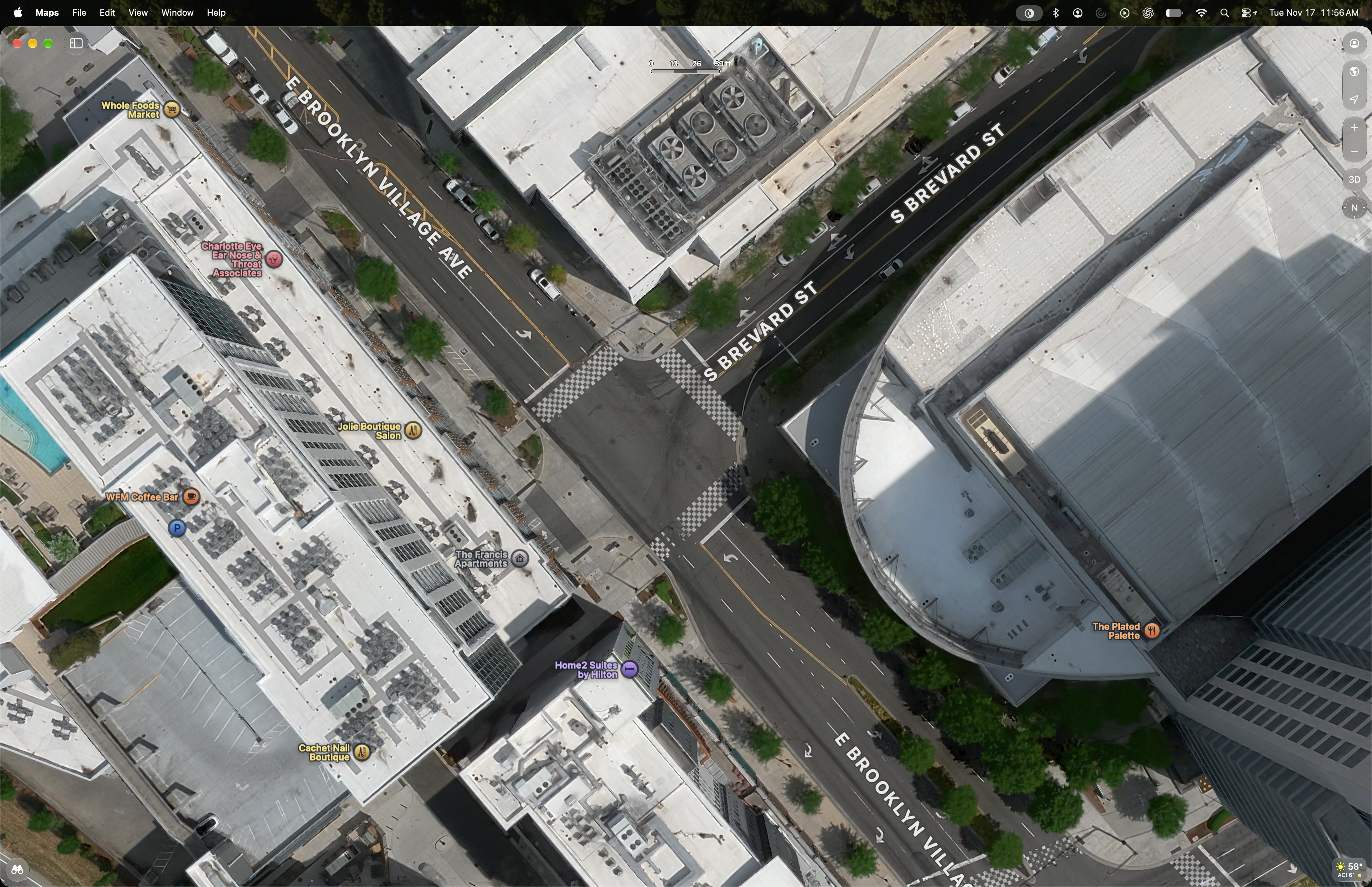
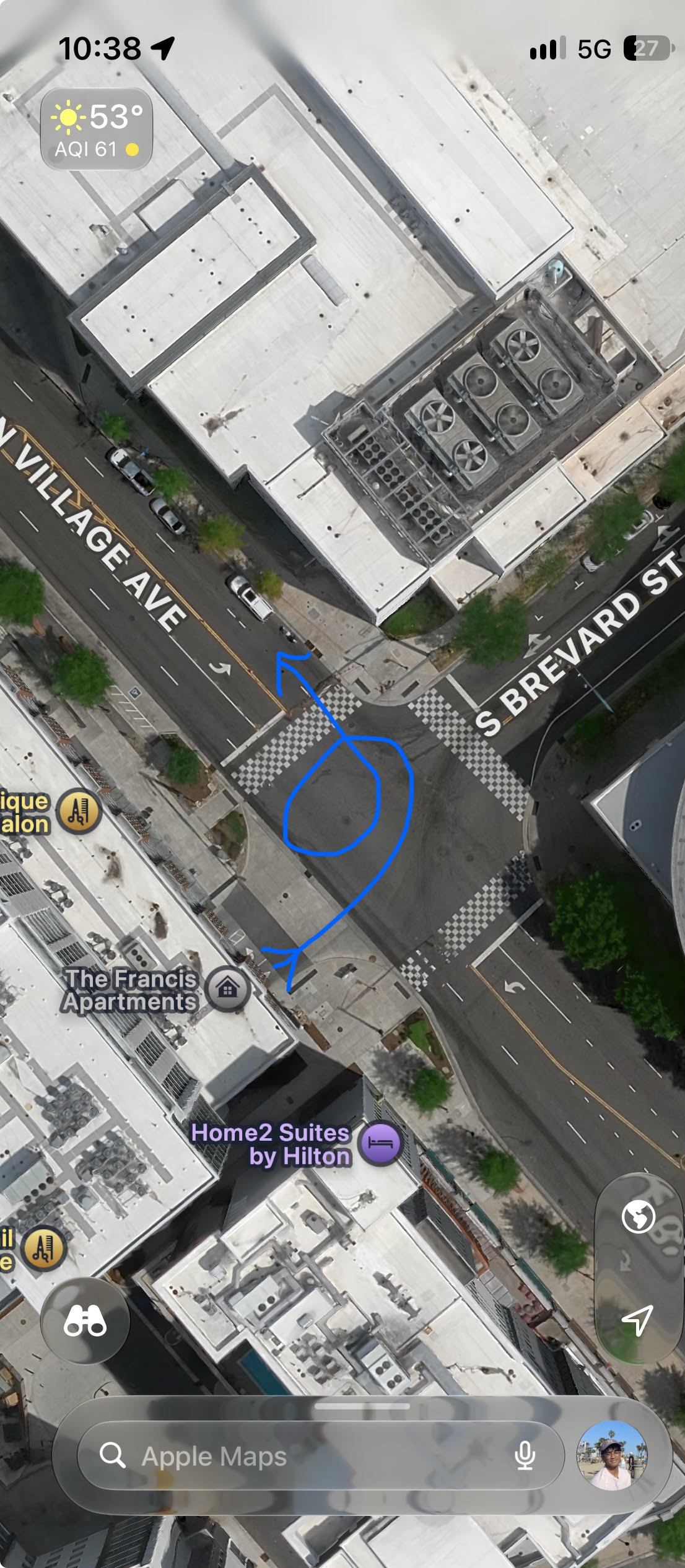
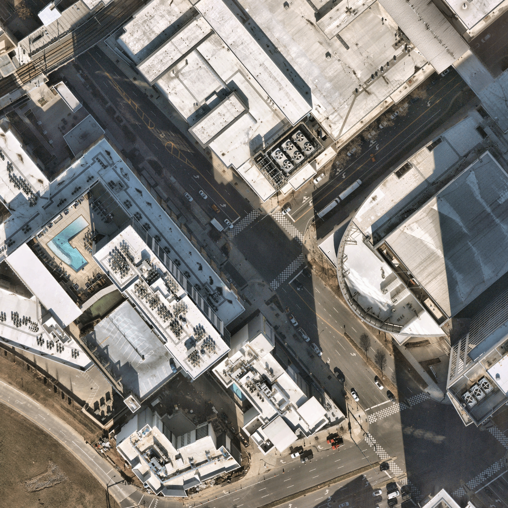
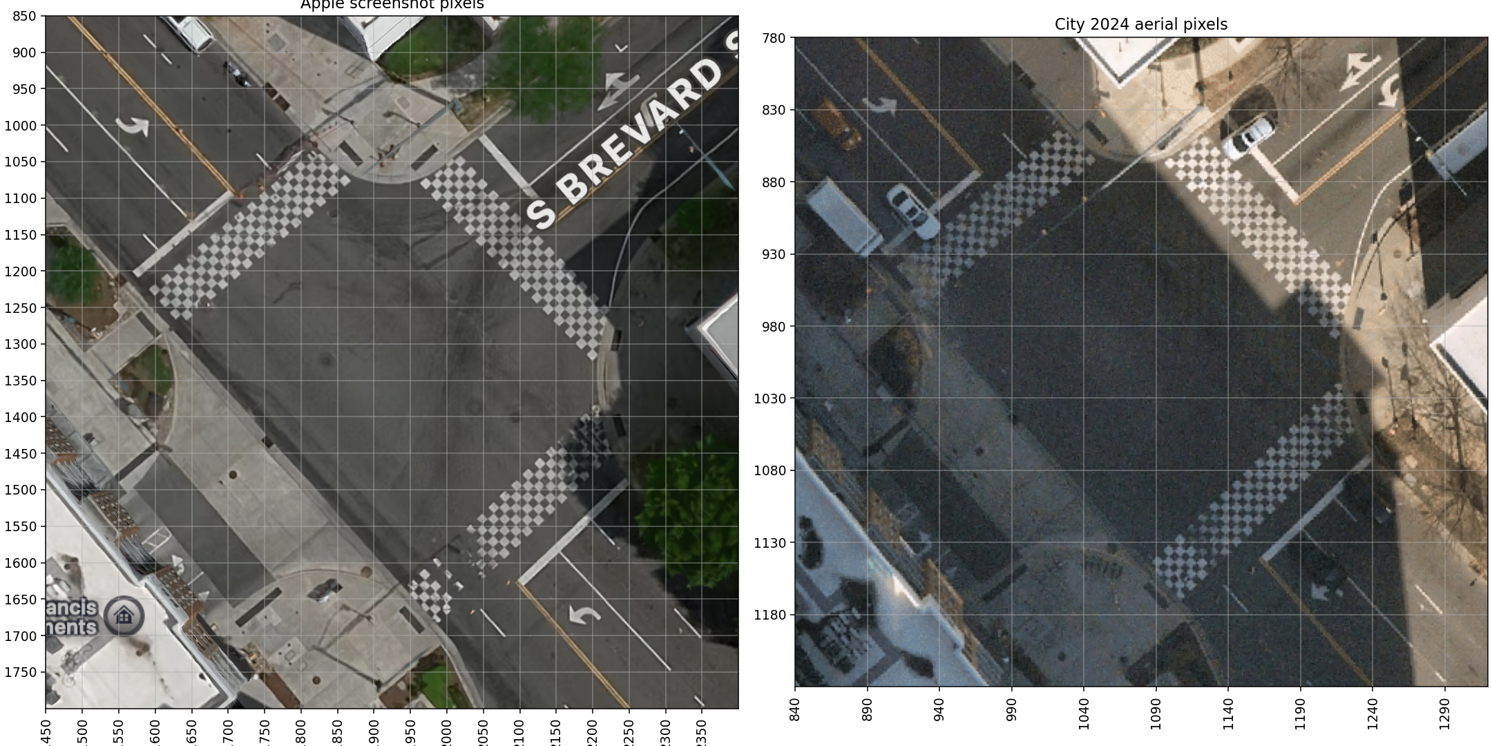
Use the actual RC F dimensions
Lexus’s 2016 specification sheet supplied the body dimensions, wheelbase, curb mass and drivetrain reference. The dimensions set the vehicle footprint on the map. Mass, wheelbase and power enter the model’s plausibility checks.
| Factory reference | Value |
|---|---|
| Engine | 5.0-litre V8 |
| Length × width | 4.705 × 1.845 m |
| Wheelbase | 2.730 m |
| Curb mass | 1,795 kg |
| Drivetrain | RWD, eight-speed automatic |
| Peak power | 467 hp |
| Peak engine torque | 389 lb-ft |
| Differential | Torsen LSD standard, TVD optional |
| Published tire sizes | 255/35R19 front, 275/35R19 rear |
The fitted differential, exact stability-control mode, tire condition and event torque remain unknown. The supplied racing-car image is a visual proxy scaled to the production RC F footprint.
Track what stays visible
The initial pipeline uses Shi–Tomasi corners, pyramidal Lucas–Kanade tracking, a forward/backward consistency check and RANSAC. I selected conservative rectangular regions around building/tree candidates and the cabin display. The wheel work estimates apparent image-plane patch rotation after cabin-display correction. Steering-wheel angle and road-wheel angle still need additional geometry.
The conservative scene filter retained 322 frame pairs, with a median of 57 inliers. A pair needs at least eight inliers and a 60% inlier fraction. The excluded interval produces no scene overlay.
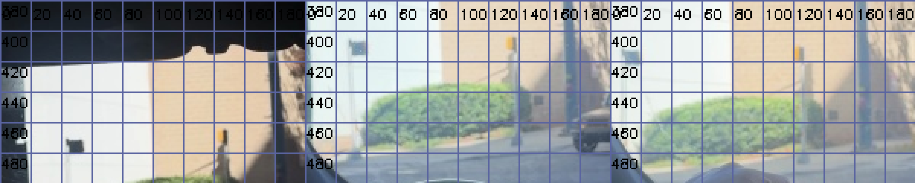
I also checked two manually labeled scene landmarks independently. The failures stayed in the record.
| Landmark | Time | Endpoint difference | Check |
|---|---|---|---|
| Dark sign | 2 s | 2.07 px | Chain passed |
| Yellow pole | 2 s | 1.34 px | Chain passed |
| Dark sign | 4 s | 1.02 px | Chain had already failed |
| Yellow pole | 4 s | 3.20 px | Beyond the provisional 3 px tolerance |
Round-trip and RANSAC checks test consistency. Independent labels still matter, particularly when the camera moves.
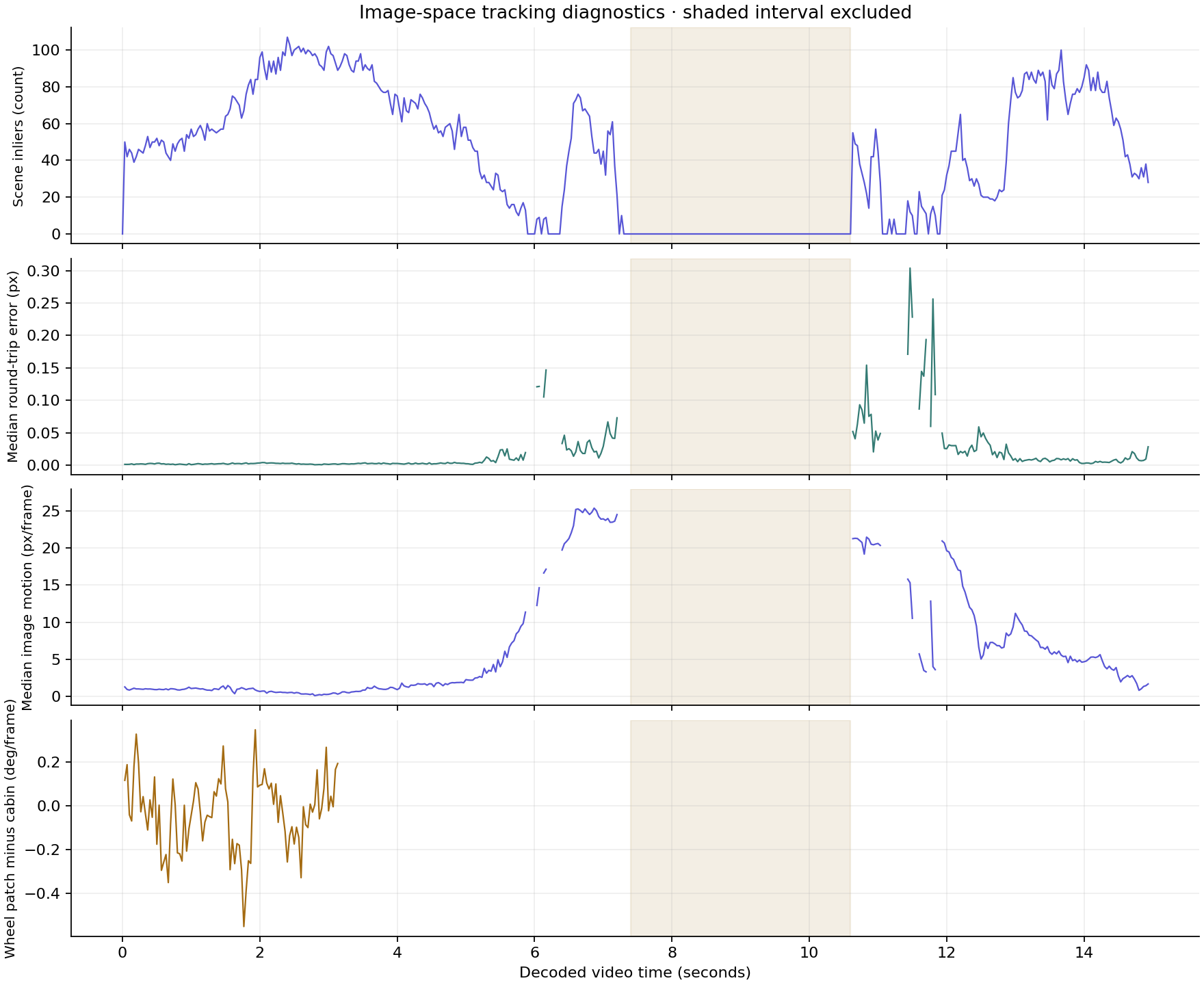
Independent labels and the annotated tracking clip
Silent diagnostic derivative. Points and vectors come from the recorded CV output; unsupported intervals stay blank.
Fit plausible motion
I used cubic splines for ground position and an independent body heading. Their derivatives supply velocity, yaw rate and acceleration. Sideslip is the difference between travel direction and body heading.
The fit balances my approximate route, a manually outlined road envelope, smooth motion, the vehicle footprint, aggregate force, yaw-moment and power limits. Weak normalized image-activity and early wheel-patch cues help with timing. Phone motion contaminates those cues, so their weight is adjustable.
Friction, payload, inertia, timing and body-rotation branch are assumptions. A broad, editable slip prior favors drifting over prolonged backward sliding. I kept a solution with that prior disabled so its effect can be inspected.
I compared nine fits. Eight passed the assumed aggregate limits; the lower-grip alternative remains available with a warning. The current counterclockwise fit uses μ = 0.9, 150 kg payload and a broad 45° peak-slip prior.
Its estimated peak speed is about 21 mph, with peak total acceleration near 0.90 g and peak absolute yaw near 101°/s. It totals roughly 439° of body rotation across the full clip. Other rotation branches remain available. These values depend on the route and modeling assumptions.
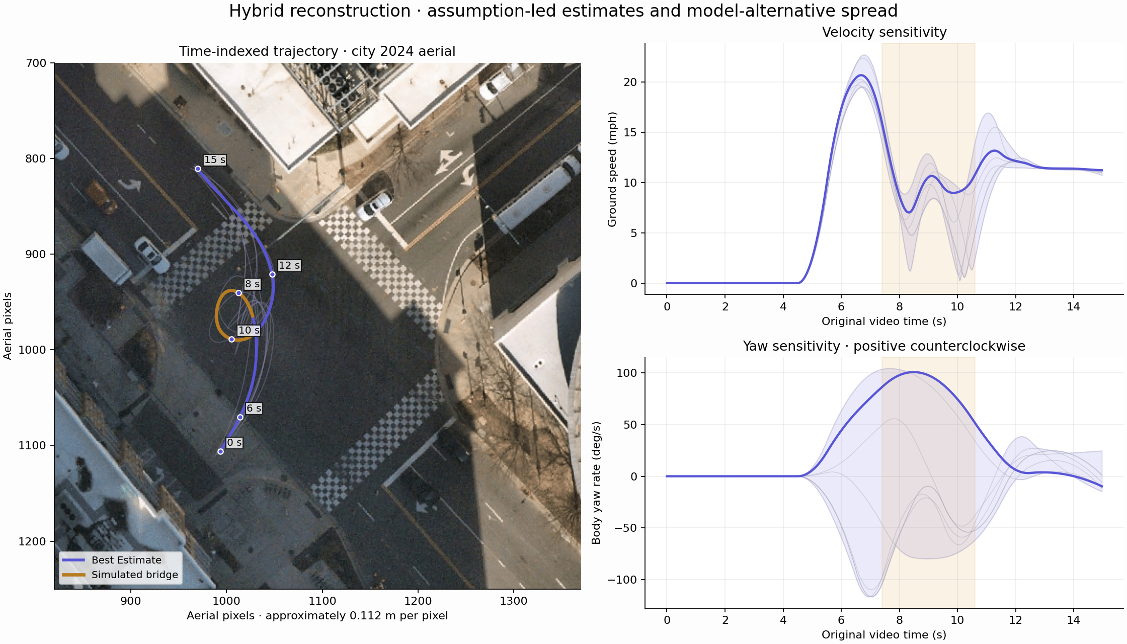
The bands show variation across the retained models. They have no statistical coverage claim. The map-alignment uncertainty also expands the displayed position envelope.
Refine it against playback
The first replay crept during the opening pause and accelerated again near the end. Reviewing it against the footage exposed both mismatches.
I made the opening state stationary through 4.5 seconds, with continuous departure derivatives. I added a 5 m/s settled exit-speed prior and a penalty against late acceleration. The revised fit eases from about 12 mph at 12 seconds to 11 mph at the end.
The retimed trajectory has about 5 m RMS deviation from the soft sketch. Its minimum modeled road clearance is around 0.3 m, which is smaller than the map-registration discrepancy. Actual curb clearance remains unresolved.
The replay uses five categories throughout: Observed, Estimated, Assumed, Simulated and Unavailable. The occluded interval is visibly Simulated. Event torque stays Unavailable, with factory specifications shown separately.
What better footage would improve
A fixed camera with a clear view of the steering wheel and road would reduce the uncertainty. Less glare and passenger occlusion would preserve more usable landmarks through the turn. Known camera geometry and an independent GPS or IMU trace would help constrain speed and body rotation.
This clip still leaves gaps. The reconstruction bridges them with explicit assumptions, and the alternative fits show how much those assumptions can change the result.
Data and reproduction
Python/PyAV handles decoding; OpenCV, NumPy, SciPy and pyproj support tracking and calibration. The trajectory solver is shared JavaScript used offline and in the browser. Matplotlib generates the diagnostics. The replay runs as static HTML, CSS and JavaScript, with the video as its master clock.
Checks cover the spline derivatives, sideslip, timestamps, stationary opening, settled exit and assumed physical limits. The source code and preserved diagnostics are available below.
Code and numerical evidence package · Official map records · Categorized time series · Full methods and assumptions
References
- Lexus Canada — 2016 RC F specification sheet. Dimensions, wheelbase, curb mass, engine, drivetrain, tires and factory peak output.
- Lexus USA — 2016 RC F product release. Production-model and differential reference.
- City of Charlotte — 2024 aerial imagery service. Georeferenced aerial export, extent and coordinate-system records.
- Esri — World Geocoding Service. Street-intersection lookup.
- Apple Maps — intersection reference. Apple Maps imagery appears in the supplied screenshots and alignment comparisons.
- OpenCV 4.10 — optical flow. Feature tracking and Lucas–Kanade reference.
- SciPy 1.14 — B-splines. Spline basis and derivatives.
I supplied the source video, map screenshots, route sketch and car artwork used for this project. The original creator of the supplied racing-car artwork was not identified. The code and numerical diagnostics were produced during this reconstruction.